Introduction

If there is no evidence of trend or seasonal effects then forecasting using demand history alone usually simply involves estimation of the demand rate (mean demand per unit time). All of the algorithms mentioned in this article can be used as a basis for forecasting involving trend and seasonal effects.

The performance of each algorithm is demonstrated using two sets of computer generated monthly demands. One set has a demand rate of 120 per year and the other set has a demand rate of 3 per year.

In the days when disk space was an expensive commodity, it was normal to use monthly demand aggregates for forecasting. It is better to use weekly demands and better still to use daily demands. All of the algorithms mentioned in this article can be used with monthly, weekly or daily demands.

 

Moving Mean

This is more commonly called a moving average. I am referring to it as a moving mean to distinguish it from a moving median.

In order to find a five month moving mean, for example, divide the total of the last five month’s demands by five.

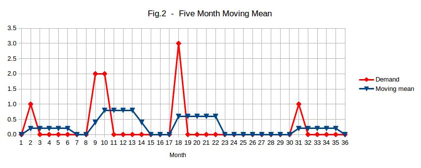
Figures 1 and 2 illustrate a five month moving mean for fast and slow moving items respectively.

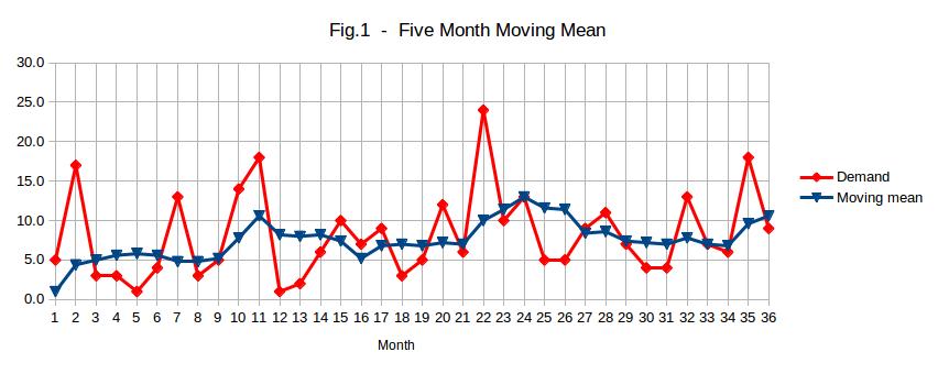
The amount of time over which the mean is taken should be long in comparison with the lead time. I suggest four times as long.

Note that, in Figure 2, the demand rate estimate is frequently zero. Such a demand rate estimate is of little use for inventory management purposes because division by zero is impossible. This will cause some inventory management algorithms to fail. A moving mean does not facilitate manual intervention in the forecasting process. The demand rate estimate increases after a relatively high demand, tending to result in over-ordering. See the article entitled “Evaluating Forecasting Algorithms” in that regard.

 

Moving Median

This is the same as a moving mean except that a median is used instead of a mean. A median is more robust than a mean, meaning that it is less sensitive to outliers (unusual monthly demands). It is an indication of what is typical.

Figures 3 and 4 illustrate a five month moving median for fast and slow moving items respectively.

 

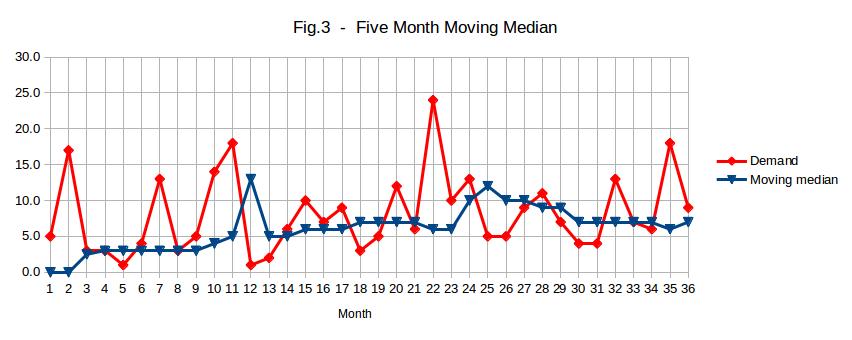
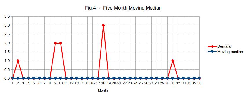
A benefit of a moving median is that relatively high demands do not, by themselves, tend to increase the demand rate estimate. This tends to avoid the over-ordering problem mentioned in relation to moving means above. Look at month 22 in Fig.3 in that regard.

Notice, from Figure 4, how inappropriate a moving median is for infrequently moving items, frequently giving zero estimates of the demand rate. It is worse than a moving mean in that regard.

Another problem with a moving median is that it doesn’t facilitate manual intervention in the forecasting process.

If sales, rather than demands, are used for estimating the demand rates then a moving median will tend to filter out the effects of promotions and lost sales provided that the median is taken over a long enough period of time. I will suggest better methods of dealing with promotions and lost sales in a later blog post.

 

Exponential Smoothing

This involves adjusting the demand rate estimate each month using the most recent month’s demand. The weighting given to the most recent month’s demand is called the “smoothing constant”. If the smoothing constant is 0.1 then 10% of the most recent month’s demand is added to 90% of the previous demand rate estimate to give the new demand rate estimate.

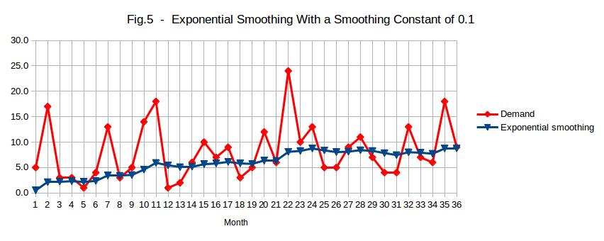
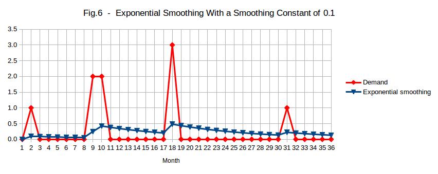
Figures 5 and 6 illustrate exponential smoothing with a smoothing constant of 0.1 for fast and slow moving items respectively.

Exponential smoothing has the following advantages compared with moving means and moving medians:

• The entire demand history is used and, as a result, the demand rate estimate will only be zero if there has never been any demand.
• Only one month’s demand needs to be stored.
• More weight is given to recent demand history than to old demand history.
• The demand rate estimate can be replaced if it is considered to be inappropriate. The estimate will be adjusted after that using subsequent demands.

The demand rate estimate increases after a relatively high monthly demand, tending to result in over-ordering. See the article entitled “Evaluating Forecasting Algorithms” in that regard. This problem can be reduced by using weekly or, better still, daily demands instead of monthly demands.

I suggest that the smoothing constant be set equal to  2/(4L+1)  or 0.1, whichever is smaller, where  L  is the lead time. The unit of measure for  L  should be months if the exponential smoothing is done monthly, weeks if it is done weekly, etc. A higher smoothing “constant” could be used initially if the initialisation of the demand rate estimate is not carried out well.

Note that, in Figure 5, the demand rate appears to be increasing. It is not. This illustrates how bad human judgement is in relation to statistical data.

A number of forecasting algorithms make use of exponential smoothing.

Because of its importance, I will discuss it in greater detail in a later blog post.

 

Croston’s Algorithm

The demand rate estimate is obtained by dividing the average demand in months in which demands occur by the average number of months from one month in which there is demand until the next. These two averages are obtained by exponential smoothing. If demands occur in one third of months and the average demand in those months is 1.2 then the demand rate estimate equals  1.2/3=0.4  per month. For items which are demanded every month, there is no difference between Croston’s algorithm and exponential smoothing.

Figures 7 and 8 illustrate Croston’s algorithm with a smoothing constant of 0.1 for fast and slow moving items respectively.

 

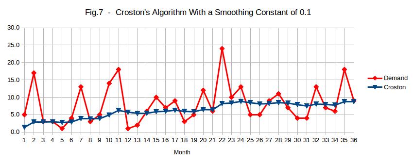
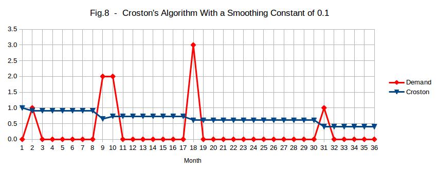
For both of the above graphs, the initial average demand in months in which demands occur was set to 1 and it was assumed, initially, that demands occur every month. In practice, it is better to carry out the initialisation on the basis of historical data.

The advantage of Croston’s algorithm over exponential smoothing is that it improves the performance for infrequently moving items. For this reason, it is often used for spare parts, most of which move infrequently.

Because of the fact that it only updates the demand rate estimate after a demand, it has an upward bias. If the demand ceases completely and never resumes then the demand rate estimate will never diminish.

 

Croston Median Algorithm

I developed this algorithm with the special needs of inventory management in mind. It combines the advantages of Croston’s algorithm with the advantages of a moving median and deals with the shortcomings of both of those techniques. This algorithm has not been published previously.

It is Croston’s algorithm with the following changes:

1. When updating the estimated mean demand per month in which demands occur, the median of the demands in the last three such months is used instead of the demand in the last such month. I suggest that the median of the last five instead of the last three be used if daily, rather than monthly demand aggregates are used.
2. When updating the estimated mean time between months in which demands occur, the median of the last three such times is used instead of the last such time. I suggest that the median of the last five instead of the last three be used if daily, rather than monthly demand aggregates are used.
3. If the time since the last month in which demand occurred is greater than the estimated mean of those times then the time since the last demand is used instead of the estimated mean time.
4. If the demand in the most recent month is greater than the existing estimate of the mean demand per month then the estimated mean demand per month is not allowed to decrease on that occasion.
5. If the demand in the most recent month is less than the existing estimate of the mean demand per month then the estimated mean demand per month is not allowed to increase on that occasion.

Change number 1 prevents a month with relatively high demand from increasing the demand rate estimate unless there is already some evidence that the demand rate has increased. This prevents the problem of over-ordering mentioned in the article entitled “Evaluating Forecasting Algorithms“. Two relatively high demand months in quick succession are treated as the minimum required evidence of the demand rate having increased. An additional benefit of this is that it is safe to use a higher smoothing constant than if ordinary exponential smoothing is used. This enables the demand rate estimate to catch up quickly with a change in the demand rate once there is substantial evidence that the demand rate has changed.

Change number 2 was made for similar reasons to change number 1.

Change number 3 enables the demand rate estimate to diminish if there has been no demand for some time, thereby reducing the likelihood of obsolete items being reordered. The demand rate estimate will pop back up again if demand resumes.

Changes 4 and 5 deal with a minor short term side effect of combining means and medians.

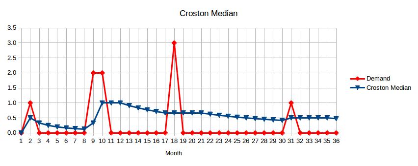
Figures 9 and 10 illustrate the Croston Median algorithm with a smoothing constant of 0.2 for fast and slow moving items respectively. A higher smoothing “constant” is used until there have been six months containing demands.

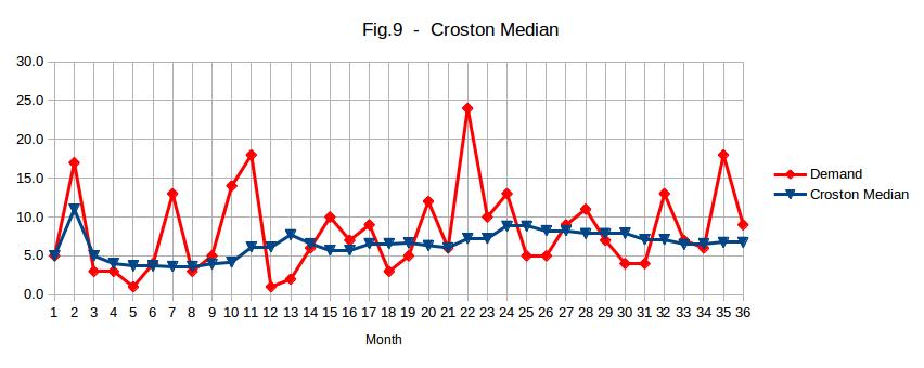
Note that Figure 9 does not give the impression of an increasing demand rate to the extent that Figure 7 does. This is because the Croston Median algorithm does a better job than exponential smoothing at recognising that the demand rate is constant.

Note that, in Figure 10, the demand rate estimate starts to diminish during a relatively long gap between demands and pops back up again when demand resumes.

The Croston Median algorithm cannot be used until there have been three periods (months in the case of the above graphs) in which demands have occurred. For this reason, the average demand to date is used until there have been three periods with demand. No algorithm can provide a satisfactory demand rate estimate with fewer than three demands.

In a later article, I will discuss the algorithm in greater depth. So far, I have only demonstrated a version designed for use with monthly demands. If weekly or, better still, daily, demand aggregates are used, much better performance can be achieved.

 

Help Available

Please feel free to contact me if you require help with implementation of a forecasting technique.