I have developed an inventory simulation spreadsheet for educational purposes. It provides two facilities which are not provided by the online simulator which is accessed by means of the “Simulator” tab. The additional facilities are graphs and use of your own demand history. The online facility is more versatile than the spreadsheet. Also, it carries out much longer simulations, thereby giving more accurate results.
Click here to obtain a copy in Open Document Format. That is a standard format which can be read using almost all modern spreadsheet software. If you are using a pre-2013 version of Microsoft Office then click here instead to obtain an Excel 97 version of the spreadsheet. That version has not been tested as thoroughly as the Open Document Format version.
You cannot use the spreadsheet online so you will need to download a copy. To do so, click on the icon with three dots near top right hand corner of the browser window and then click “Download”.
If you encounter any problems then please contact me and let me know what spreadsheet software you are using. You are least likely to encounter problems if you use Libre Office which is a free download.
The yellow cells are the cells in which you can enter data.
Cell E4 should contain the number of the forecasting algorithm which is to be used. At present it should contain 1 which is exponential smoothing. The Croston, Croston Median and Holt-Winters algorithms are to be added later.
In Cell E5, enter the desired smoothing constant for exponential smoothing. The smoothing constant is the weighting to be given to the most recent period’s demand and should be between 0 and 1.
In Cell E6, enter the lead time in periods starting from when the order is sent to the supplier. It must be 1 or 2 or 3 or 4 or 5 because of the limitations of spreadsheets. The length of a period can be anything you like (e.g. month or week or day). At the beginning of each period, if the inventory position is strictly less than the reorder point then an order is sent to the supplier to increase the inventory position to the “maximum” level. The inventory position is the quantity on hand minus the quantity on customer back order plus the quantity on supplier order. The lead time is treated as being deterministic (fixed). If you want to use stochastic (varying) lead times then you will need to use the online simulator.
In Cell E7, enter the reorder point expressed as a number of periods supply,
In Cell E8, enter the “maximum” level expressed as a number of periods supply. It should not be less than the entry in cell E7.
In Cell E9, enter the mean demand per period to be used when the spreadsheet is used to carry out Monte Carlo simulations.
If no entries are made in Column C, Monte Carlo simulations will be carried out. Changing the contents of a yellow cell or re-entering what is already there will result in a new Monte Carlo simulation. If you want simulations to be carried out using your own demand history, enter that history in the yellow cells in Column C, starting from the oldest period. Deleting Cell C12 will result in a return to Monte Carlo simulation. The Monte Carlo simulation of demands is carried out in the same manner as in the online simulator.
In Cell D12, enter the assumed initial estimate of the mean demand per period.
In Cell E12, enter the assumed starting inventory level (stock on hand minus the quantity on customer back order).
Columns E to J show the situation at the beginning of each period.
The estimated mean demand per period is updated, using exponential smoothing, at the end of each period
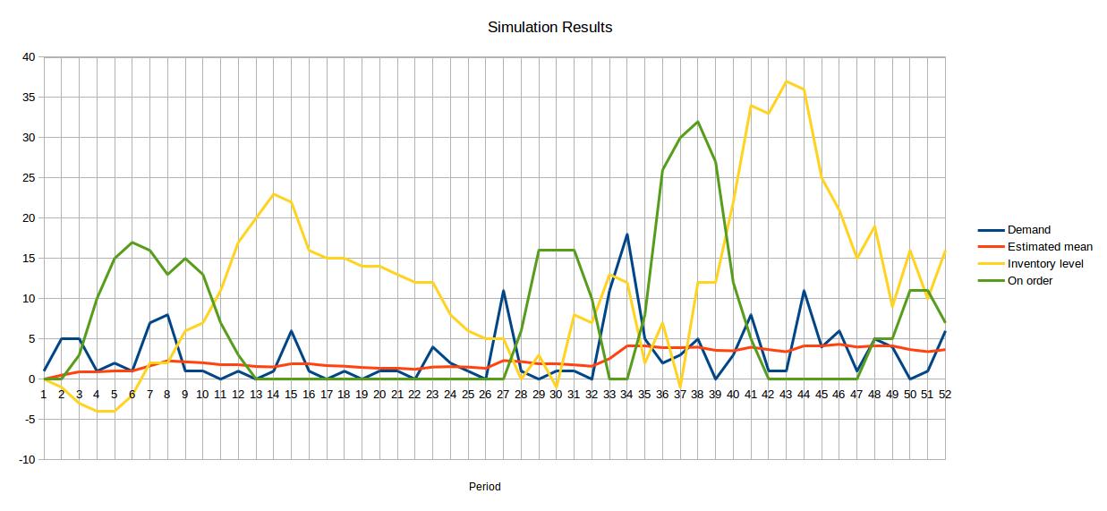
The results of the simulation are shown in the two graphs and in cells L5 to P6.
Recent Comments